Finite Elements Method, volume and discrete elements: which are the main differences?
In order to assist the engineering problem-solving challenges, there are several numerical simulation methods, each of which containing particularities and specific applications. The Finite Elements Method evolved through the improvement of the structural analyzes, such as using reticulated models (mainly in the aeronautic industry) and the development of computer usage, especially circa mid 50s according to some sources.
On the other hand, the Finite Volume Method (FVM) is preferred by professionals who constantly deal with fluid mechanics, it can also be used to solve problems involving heat or mass transfer. Discrete Element Method (DEM), in turn, is widely applied in granular flows.
Acknowledging the theory behind the mathematical and computational models is essential to better understand its operational issues and seek solutions for recurrent engineering issues. This article introduces you to the three methods mentioned: FEM, FVM, and DEM.
Finite Elements Method (FEM)
Initially, the FEM was used in the study of problems in the mechanics of solids (for the evaluation of stresses in aircraft wings). In a short time, it was extended to applications involving other physical phenomena, making it a method widely applied in industry and academia. It evolved from static to dynamic analyzes; from linear to non-linear problems; from a single phenomenon to several simultaneous that interact with each other.
The finite element method uses the discretization of the system in several elements to solve differential equations, replacing an infinite number of variables with a limited number of elements of known behavior. The elements are of finite dimensions, giving rise to the method name.
According to the type and dimensions of the problem, different forms of the divisions might occur. From these we defined the nodes and meshes:
- Nodes: nodes are finite elements connected by points and can move according to the loading application, thus providing answers about the studied phenomenon.
- Mesh: the number of nodes will represent the number of unknown factors that the problem will have and its sum is known as mesh.
This methodology solves the mathematical equations using approximations due to the subdivisions of the geometry, so choosing the appropriate mesh is very important for the quality of the results. Its precision is related to the quantity and size of the nodes and elements, the quality of the mesh, and the type of function used. For better precision, the smaller the area of the element must be and the greater the number of nodes and elements in the mesh. However, a very large number of elements leads to an increase in the rounding error, which may impair the accuracy of the result and computational power consumption.
In short, the geometry of what you want to analyze is divided into elements, which are small parts that represent the continuous domain of the problem. In this way, it is possible to develop the structural analysis by means of displacements, deformations, and stresses. It is also possible to simulate various scenarios and, thus, estimate the performance of a given product in relation to strength, stiffness, and fatigue.
In other words, the Finite Element Method allows us to identify if a product or component analyzed meets the required standards, observe the points of concentration of tension and understand the behavior of the structure before a load. Therefore, the FEM allows the geometry improvement of the object even before its manufacture.
Technology can allow the integration between software used to create the geometric representation, called CAD (Computer Aided Design), and the software used to solve the problem based on the Finite Element Method, called CAE (Computer Aided Engineering), leaving the faster and more efficient analyzes.
The stages for the analyzes of the Finite Elements Method are listed below:
- Build the CAD model of the system being analyzed;
- Determine the material’s properties;
- Build a mesh of the model in the CAE software;
- Determine the loads and the restricting conditions;
- Seek a solution;
- Analyze the results.
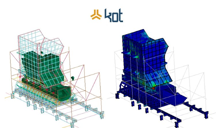
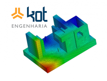
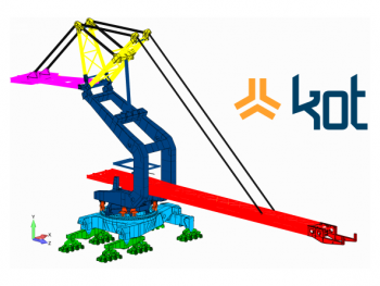
An implementation example of Finite Elements conducted by Kot can be seen on Figure 1.
Finite Volume Method (FVM)
When it comes to the study of fluids, one must obey the fundamental laws of physics with regard to the conservation of mass, amount of movement, and energy. These fundamental laws lead us to the continuity, energy, and Navier-Stokes equations. This crack is commonly called the Navier-Stokes equations, a set of equations composed of partial derivatives that describe the behavior of fluids.
The most applicable numerical method for solving flow problems is the Finite Volume Method. In this, the domain is decomposed into control volumes (CVs) to allow the study of fluids. You can divide the FVM, used in CFD (Computational Fluid Dynamics) software into three steps:
- FVM pre-processing
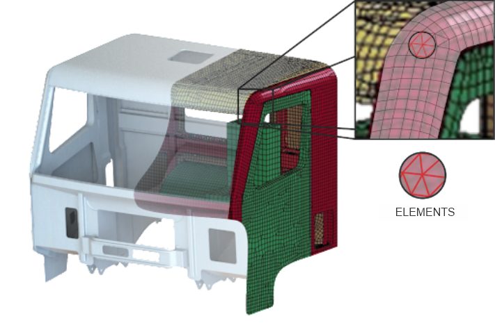
Initially, the geometry to be worked must be constructed. Then, the domain is subdivided into smaller parts, generating a mesh of cells, called control volumes (Figure 2). Material/fluid properties are also identified and boundary conditions are included.
- FVM Simulation
Here, the Navier-Stokes equations are applied to each of the control volumes. Physical models of turbulence, combustion, radiation, etc. are analyzed using numerical equations. Conservation of mass, amount of movement, energy, and other equations and transport variables determine the conditions of the simulation. The entire calculation is performed based on the approximation of the variables involved and, once the system of equations is ready, it will be solved according to the demand of each case, in a segregated or coupled way.
- FVM post-processing
The results of the analyzes are presented in graphs and tables. When using the tools, the distribution of vectors in the geometry and the profile of the contour distribution can also be obtained. Thus, what was previously subdivided into control volumes, is now analyzed globally.
Although the finite volume method has similar characteristics to FEM, FVM is the most suitable and usual for fluid dynamics simulations. This is because the laws of thermo fluid dynamics are best applied to control volumes, especially in problems related to multiphase, reactive, turbulent, or more complex flows.
Discrete Elements Method (DEM)
The Discrete Element Method (DEM) is used when it is desired to calculate the flow, movement, or dynamics of a large number of discrete particles. It covers both computational methods that allow the analyzes of the displacements and rotations of discrete bodies, as well as methods that automatically recognize new contacts as the calculations and iterations are performed.
The analysis starts from the description of the individual movement of the particles in each increment of time. The displacement of the particles is given by the general equation of Newton’s motion and the Euler equation for rotations. Knowing the movement, the boundary and/or operating conditions are established and it is possible to reach the desired result.
DEM is notably applied in the numerical simulation of granular material flows with or without comminution. Among the main applications, it is possible to mention:
- Multiphysical models which include granular flows;
- Complex particle shapes, in two or three dimensions;
- Complex movements with particles of different sizes interacting with each other;
- Particle break models (like ore crushers);
- Predict the probability of particle breakdown from the energy spectrum;
- Simulation of surface wear.
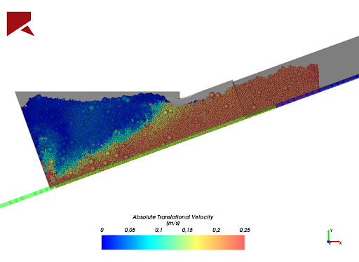
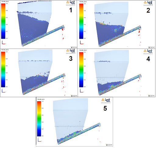
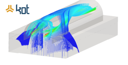
In Figure 3, it is possible to analyze the representation of the discrete particles in a software that uses DEM.
When to use FEM, FVM, and DEM?
In general, FEM is used in structural analysis, FVM covers flow simulations and fluid behavior and DEM is applied for the movement of discrete particles.
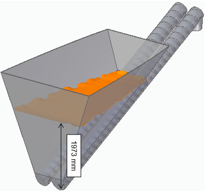
A practical example would be the study of a silo in which fruit peels run out. In this case, the stored and drained material presents a great variation in its physical parameters, which are affected, among other things by: variations in the harvest period, fruit variety, previous processes and time spent in transportation. It is possible to know the behavior of each material in the silo and its interference in the metallic structure.
When the fruit peels are dry, their flow must be determined by the discrete element method. Thus, it is possible to identify clogging regions, material accumulation, asymmetric flow, among other common interferences in this type of operation. This example can be seen in Figure 4.
Additionally, in the condition of the material in which there is high humidity and the shell presents itself as a viscous material, its flow is determined by the finite volume method. In this situation, it is possible to observe, for example, how the viscosity of the fluid interferes with the flow and what are the impacts generated. See an example in Figure 4.
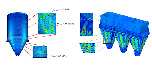
From the DEM and FVM/CFD analysis, it is also possible to obtain the loads that the material, under operating conditions, imposes on the silo structure. Thus, a FEM analysis must be made with these loads as boundary conditions, as shown in Figure 6.
There are several ways to apply numerical methods. It is essential to understand the theory behind each one in order to carry out computational studies that can actually add value, solving everyday problems that challenge the industry.
Get in touch with KOT’s specialists team!

Aender Ferreira
Mechanical Technician from CEFET-MG, Mechanical / Aeronautical Engineer from UFMG and Master in mechanical projects from the same university. Before graduation, he had experiences in the mining, maintenance, project design, experimental engineering and automotive industries. As an Engineer, he started his career in the maintenance sector performing calculus activities for fatigue in aeronautical components and structures. Subsequently, he was invited to compose the Board of Directors of KOT Engineering, working in the commercial sector of the company, helding the position for almost 15 years.
Reference:
Malalasekera, W., and H. K. Versteeg. “An introduction to computational fluid dynamics.” The finite volume method, Harlow: Prentice Hall (2007): 1995.


Leave a Reply