In general, three methodologies stand out in the search for solutions to engineering problems: analytical methods, experimental methods, and numerical methods. First and foremost, to understand numerical methods, one must be familiar with the other methodologies used. Throughout this article, we will introduce the concepts behind these three methods and explore the use of numerical methods in solving engineering problems. 

Analytical Method 

In general, the Analytical Method is used for less complex problems. It is a simple methodology that provides a direct answer by solving—usually manually—equations based on mathematical formulas, in which input variables are defined to determine the values of the output variables. 

However, analytical calculations cannot be applied to all engineering challenges, since solving the equations that describe the phenomenon under study can be too complex to compute—for example, solving second-order, nonlinear partial differential equations. For this reason, to make the equations solvable, the physical characteristics describing the phenomenon are simplified, making them much simpler than what is observed in practice. As a result, the product obtained from the analytical solution of the equations may deviate significantly from the actual product, leading to oversizing issues, which increase the cost of production or implementation of a project.

However, the analytical solutions of simple problems can be used as a basis for understanding the behavior of the system of equations, for developing numerical methods and for verifying computer codes.

For example, a collision between two bodies can be classified as elastic when the system’s energy and linear momentum are conserved, as described by the equation shown in Figure 1. However, most collisions found in nature cannot be classified as elastic; this assumption is a simplification used to facilitate application in specific cases.

 

Figure 1: Law of Conservation of Motion in an elastic shock
- using the analytical method - SOURCE: Kot Collection.

 

Experimental Methods

In addition, experimental methods use physical prototypes—which may be full-scale or scaled-down—to study the phenomenon. Tests are conducted to simulate the operating conditions of that product. Classic examples of the application of this methodology include a car crash test or the aerodynamic analysis of a Formula 1 car in a wind tunnel, as shown in Figure 2 [1].

 

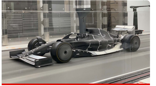
Figure 2: Formula 1 car simulation for the 2021 season using the "wind tunnel" experimental method - SOURCE: BARRETTO (2019).

 

Experimental methods yield high-quality results and provide a detailed understanding of the phenomenon under study; however, they require a significant investment. This investment is not limited to the cost of building the prototype but also includes the resources needed to establish the infrastructure essential for accurately simulating the physical operating characteristics. Similarly, another challenge encountered when using the experimental method is the time required to set up the test, since it may be necessary to perform multiple simulations or long-duration simulations and build different prototypes until an optimal design is achieved, particularly in destructive testing. Finally, some real-world conditions cannot be reproduced; for example, the simulation of oil reservoirs [2]. 

Numerical method

Unlike previous methods, the numerical method finds approximate numerical solutions to a wide variety of complex real-world problems by applying algorithms that make it possible to formulate and compute mathematical operations using sequences of simpler arithmetic operations. numerical analysis and designs methods to efficiently find solutions to mathematically expressed problems” [3]. 

In this context, an algorithm is a finite set of ordered operations that enables the solution of a specific problem. It consists of a series of specific instructions that, through a sequence of steps, make it possible to find an approximation of the result.

Furthermore, numerical analysis to find an approximate solution to the actual value through sequences, using as few elementary operations as possible. Although it originated before the advent of computers, it is now associated with information technology. As computers became more affordable and gained greater processing power, the use of computational methods and techniques became widespread for solving real-world problems where manual solutions might be impractical, inaccurate, or require a significant financial investment or a long execution time. 

Consequently, the numerical method is an approach that, although it requires a greater investment than the analytical method—due to the need for hardware infrastructure and software licenses—still requires a smaller investment than the experimental method. Nevertheless, it is an approach that, even when using assumptions that simplify the phenomenon compared to what is observed in reality, still makes it possible to obtain a representation similar to that found in the study of a physical prototype in a shorter amount of time. 

A practical application of numerical methods, for example, is CFD simulation , which, based on the laws of thermofluid dynamics, seeks to solve the defined problem using computational resources. In the example shown in Figure 3, the CFD technique can be used to determine the pressure distribution across the entire outer surface of a vehicle, thereby calculating aerodynamic coefficients of drag and downforce, at a considerably lower cost than wind tunnel testing.

 

Figure 3: CFD simulation to define the best aerodynamic profile - SOURCE: Kot Collection.

 

Numerical solution

In general, to solve a problem using numerical solutions, one must follow a few steps, as shown in Figure 4 [3].

 

Figure 4: Steps involved in the numerical solution of a physical problem - SOURCE: FRANCO (2011).

 

First, the mathematical model must be developed based on observations of the phenomenon, using the laws of physics and mathematics. It must be constructed in such a way that it accurately represents the actual physical characteristics of the problem.

Next, the mathematical model is used to obtain the numerical model using the method of approximations. This methodology is based on discretizing the domain and solving the differential equation at specific points.

Thus, the necessary steps in the numerical solution can be summarized as follows: 

Physical Model > Mathematical Model > Numerical Model > Numerical Solution > Numerical Results.

Therefore, care must be taken at every stage of solving the problem under analysis to ensure that the numerical solution accurately represents the physical phenomenon being modeled. Otherwise, meaningless solutions may be obtained. “A numerical tool is appropriate and reliable when one has a numerical method that correctly solves the differential equations and a mathematical model that accurately represents the physical phenomenon.” [3]. 

In addition, the numerical solution may contain two types of errors when the results are compared with the actual physical problem. Numerical errors result from incorrectly solving the differential equations. In this case, it is necessary to compare the result with other analytical or numerical solutions. On the other hand, there are also errors arising from the use of equations that do not correctly describe the phenomenon under study.

Conclusion

In summary, numerical methods have several advantages over other methodologies, including: 

• • Low cost compared to the experimental method;

• • Shorter problem-solving time;

• • Easy to simulate realistic conditions.

However, the numerical solution should not be viewed as a substitute for other methods. Therefore, it is the engineer’s responsibility to analyze and determine the best methodology for solving the problem, taking into account the advantages and limitations of each method.

Kot Engenharia the experience and resources necessary to evaluate and define the best methodologies to be used to boost your business. Consult our team for more information!

Follow our pages on LinkedIn, Facebook e Instagram to keep up with our content.

References: 

[1] BARRETTO, Lawrence. First Look: Formula 1’s 2021 car in the wind tunnel. Formula 1, 21 de agosto de 2019. Disponível em: <https://www.formula1.com/en/latest/article.first-look-formula-1s-2021-car-in-the-wind-tunnel.6ye3S7Pb8NRX1K7PjTBxtS.html> Acesso em: 11 de abril de 2020. 

[2] FRANCO, Admilson T. Métodos Numéricos Aplicados à Engenharia: Introdução aos métodos de diferença finitas e de volumes finitos. 2011. 9 f. Mechanical Engineering Course, Academic Department of Mechanics, Federal University of Pará, Curitiba, 2011. Chap. 1.

[3] ARAÚJO, Eduardo. Métodos Numéricos para Simulação na Engenharia. Blog ESS, 30 de novembro de 2017. Disponível em <https://www.esss.co/blog/simulacao-numerica-metodo-analitico-experimental-concorrentes-ou-complementares-na-engenharia/.>  Acesso em: 20 de setembro de 2020.