There are various numerical simulation methods for solving engineering challenges, each with its own particularities and main applications. The aim of this article is to present the main differences between these methodologies, as described below. The use of the finite element methods (Finite Element Method - FEM) has evolved with improvements in structural analysis. As an example, we can cite the use of lattice models (mainly for the aeronautical industry) and the evolution in the use of computers, mainly in the mid-1950s according to some authors.
The finite volume method (Finite Volume Method - FVM) is preferred by professionals who need to deal with fluid mechanics, and can also be used to solve problems involving heat or mass transfer. The Discrete Element Method (Discrete Element Method - DEM), on the other hand, is widely applied to granular flows.
Knowing the theory behind mathematical and computational modeling is essential to better understand operational problems and how to find solutions to common engineering problems. In this article, learn about the differences between the three methods mentioned: FEM, FVM and DEM.
Finite element method (FEM)
Evolution and Fundamentals of FEM
Initially, FEM was used to study problems in solid mechanics (to evaluate stresses in airplane wings). It soon spread to applications involving other physical phenomena, making it a method widely applied in industry and academia. It has evolved from static to dynamic analysis; from linear to non-linear problems; from a single phenomenon to several simultaneous ones that interact with each other.
The finite element method uses the discretization of the system into several elements to solve differential equations, replacing an infinite number of variables with a limited number of elements of known behaviour. The elements have finite dimensions, giving rise to the method's name.
Knots, meshes and precision in analysis
Depending on the type and size of the problem, you can have different division shapes. In these, we define nodes and meshes:
- Nodes: the nodes are the finite elements connected to each other by points and can move according to the application of load, thus providing answers about the phenomenon studied.
- Mesh: the number of nodes will represent the number of unknowns that the problem will have and their sum is known as the mesh.
This methodology solves the mathematical equations using approximations due to the subdivisions of the geometry, so choosing the right mesh is very important for the quality of the results. Its accuracy is related to the number and size of nodes and elements, the quality of the mesh and the type of function used. For best accuracy, the smaller the element area and the greater the number of nodes and elements in the mesh. However, a very large number of elements leads to an increase in the rounding error, which can affect the accuracy of the result and the consumption of computing power.
In short, the geometry of what you want to analyze is divided into elements, which are small parts that represent the continuous domain of the problem. In this way, structural analysis can be carried out using displacements, deformations and stresses. It is also possible to simulate various scenarios and thus estimate the performance of a given product in terms of strength, stiffness and fatigue.
In other words, the finite element method makes it possible to identify whether an analyzed product or component meets the required standards, to observe the points of stress concentration and to understand the structure's behavior under load. Therefore, FEM makes it possible to perfect the geometry of the object even before manufacturing.
Applications of the Finite Element Method (FEM) and Integration with CAD and CAE Software
Technology can enable integration between the software used to create the geometric representation, known as CAD(Computer Aided Design), and the software used to solve the problem based on the finite element method, known as CAE(Computer Aided Engineering), making analysis faster and more efficient.
The steps for finite element method analysis are listed below:
1. Build the CAD model of the system under analysis;
2. Determine the material's properties;
3. Build the model mesh in CAE software;
4. Determine the loads and restriction conditions;
5. Search for a solution;
6. Analyze the results.
An example of Kot's application of finite elements can be seen in Figure 1.
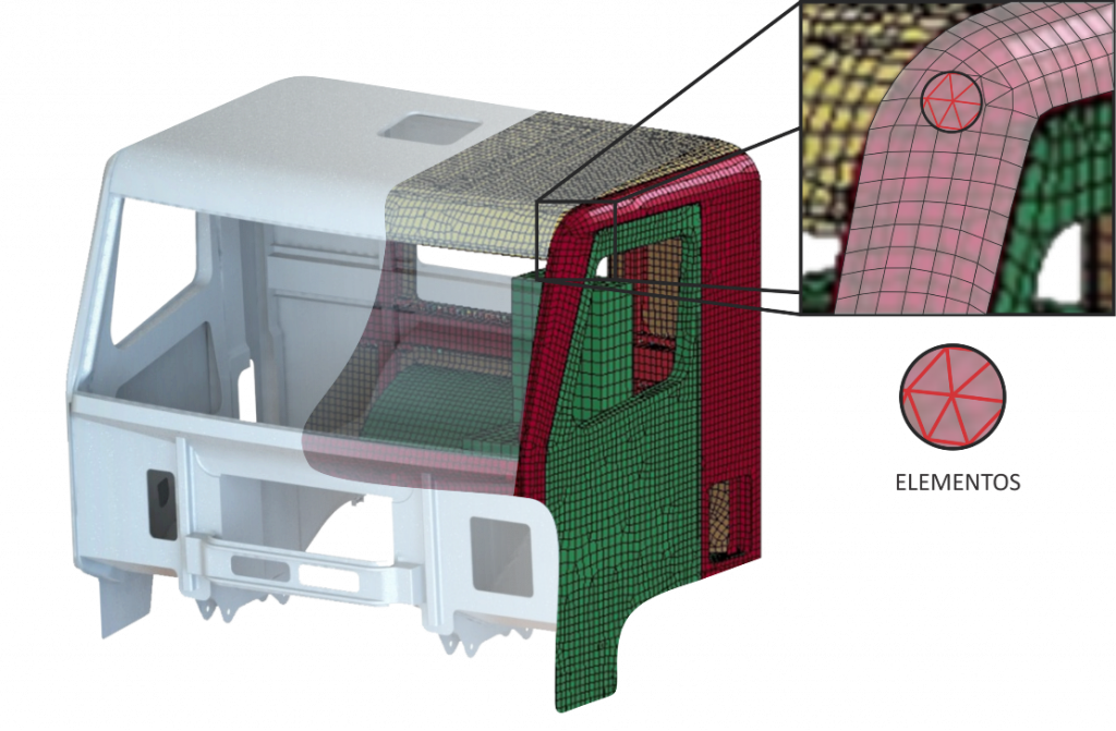
Figure 1: Practical application of mesh construction with finite element details - SOURCE: Kot Collection.
Finite Volume Method (FVM)
Fundamentals of FVM and the Navier-Stokes Equations
When it comes to studying fluids, the fundamental laws of physics regarding the conservation of mass, quantity of movement and energy must be obeyed. These fundamental laws lead us to the continuity, energy and Navier-Stokes equations. These are commonly referred to as the Navier-Stokes equations, a set of equations composed of partial derivatives that describe the behavior of fluids.
The most applicable numerical method for solving flow problems is the finite volume method. In this method, the domain is decomposed into control volumes (CVs) to allow the study of fluids. The FVM, used in CFD software(Computational Fluid Dynamics) software, into 3 steps:
Simulation steps with FVM
1. FVM pre-processing
Initially, the geometry to be worked on must be constructed. The domain is then subdivided into smaller parts, generating a mesh of cells called control volumes (Figure 2). The material/fluid properties are also identified and the boundary conditions are included.
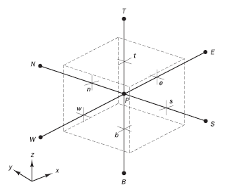
Figure 2: Representation of a control volume - SOURCE: Versteeg and Malalasekera, 1995.
2. FVM simulation
Here, the Navier-Stokes equations are applied to each of the control volumes. Physical models of turbulence, combustion, radiation, etc. are analyzed using the numerical equations. Conservation of mass, quantity of movement, energy and other transport equations and variables determine the simulation conditions. The entire calculation is carried out based on the approximation of the variables involved and, once the system of equations is ready, it is solved as required in each case, either separately or coupled.
3. FVM post-processing
The results of the analysis are presented in graphs and tables. Using the tools, the distribution of vectors in the geometry and the contour distribution profile can also be obtained. Thus, what was once subdivided into control volumes is now analyzed globally.
Although the finite volume method has similar characteristics to the FEM, the FVM is the most suitable and usual method for fluid dynamics simulations. This is because the laws of thermofluid dynamics are best applied in control volumes, especially in problems related to multiphase, reactive, turbulent or more complex flows.
Discrete element method (MED/DEM)
The discrete element method (MED) is used when you want to calculate the flow, movement or dynamics of a large number of discrete particles. It encompasses both computational methods that allow the analysis of displacements and rotations of discrete bodies, and methods that automatically recognize new contacts as calculations and iterations are performed.
The analysis starts by describing the individual movement of the particles in each time increment. The displacement of the particles is given by Newton's general equation of motion and Euler's equation for rotations. Once the movement is known, the boundary and/or operating conditions are established and the desired result can be achieved.
DEM is widely used in the numerical simulation of flows of granular materials with or without comminution. Its main applications include:
- Multiphysics models that include granular flows;
- Complex particle shapes, in two or three dimensions;
- Complex movements with particles of different sizes interacting with each other;
- Particle breaking models (such as ore crushers);
- Predicting the probability of particle breakage from the energy spectrum;
- Simulation of surface wear.
Figure 3 shows the representation of discrete particles in software using DEM.
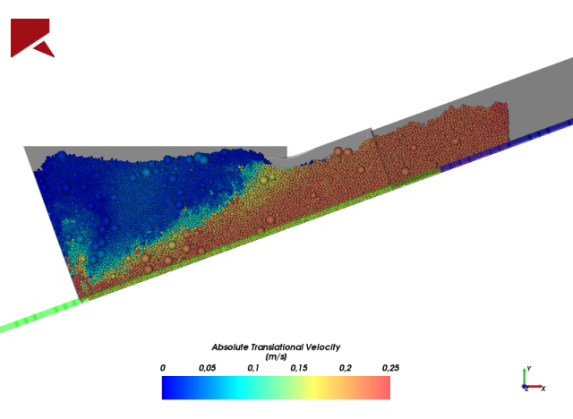
Figure 3: Representation of discrete particles in a model - SOURCE: Kot Collection.
When to apply the FEM, FVM and DEM?
In general, FEM is used for structural analysis, FVM covers flow simulations and fluid behavior, and DEM is applied to the movement of discrete particles.
A practical example would be the study of a silo in which fruit peels are being transported. In this case, the material stored and drained varies greatly in its physical parameters, which are affected, among other things, by: variations in the harvest period, variety of fruit, previous processes and time spent in transportation. It is possible to know the behavior of each material in the silo and its interference with the metal structure.
When fruit peels are dry, their flow must be determined using the discrete element method. In this way, it is possible to identify areas of clogging, material accumulation, asymmetric flow, among other common interferences in this type of operation. This example can be seen in Figure 4.
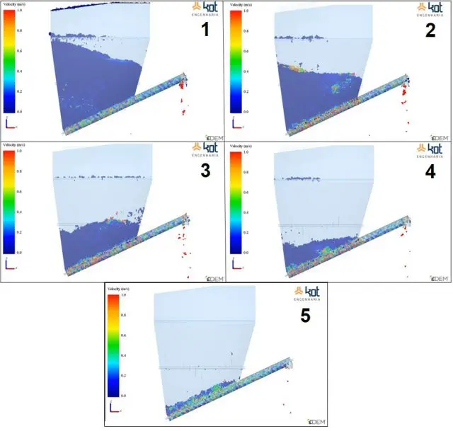
Figure 4: Flow of dry shells in a silo - SOURCE: Kot Collection.
In the case of a material with high humidity and a viscous shell, its flow is determined using the finite volume method. In this situation, it is possible to see, for example, how the viscosity of the fluid interferes with the flow and what impacts are generated. See Figure 5 for an example.
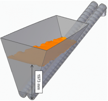
Figure 5: Height of the remaining viscous fluid level in a silo - SOURCE: Kot Collection.
From the DEM and FVM/CFD analyses, it is also possible to obtain the loads that the material imposes on the silo structure under operating conditions. An FEM analysis must therefore be carried out using these loads as boundary conditions, as shown in Figure 6.
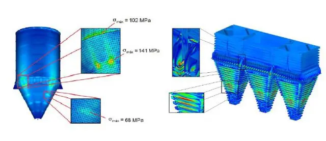
Figure 6: Finite element analysis of a silo - SOURCE: Kot Collection.
It is also possible to carry out analyses that allow the results of 2 or more methods to be viewed simultaneously. This is the case of an avalanche analysis carried out by Kot, shown in the video. In it, you can see the flow calculated using the finite volume method, while the structural analysis due to the avalanche is calculated using the finite element method.
Reference:
Malalasekera, W., and H. K. Versteeg. "An introduction to computational fluid dynamics." The finite volume method, Harlow: Prentice Hall (2007): 1995.
Numerical simulations are with Kot Engenharia
There are many ways of applying numerical methods. It is essential to understand the theory behind each one in order to carry out computational studies that can add real value by solving everyday problems that challenge industry.
If you, like our more than 150 clients, are looking for structural engineering solutions for your operation, contact our team and find out more about our services. Since 1993, we have specialized in developing engineering solutions through inspections, technological tests and the use of computer methods for complex assessments of concrete and metal structures and industrial equipment.
Follow our pages on LinkedIn, Facebook e Instagram to keep up with our content.